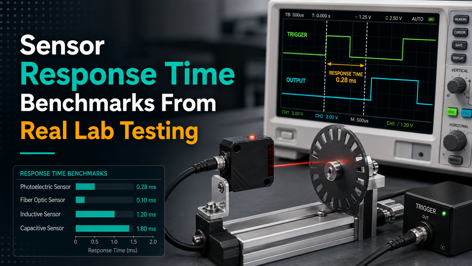
Sensor Response Time Benchmarks From Real Lab Testing

Sensor response time is the delay between an actual change in the measured quantity and the moment the sensor reports it, most commonly quantified as T90—the time needed to reach approximately 90%^[1] of the final reading after a step input. For example, fast optical sensors hit T90 in under 100 milliseconds, while some gas sensors require 30 seconds or more. Related metrics include T63 (approximately 63% of final value) and rise time, each defining sensor speed differently.

What does T90 mean compared to T63 and rise time? And which sensor types are generally the fastest? What tends to slow a sensor down, and how do the 2025,2026 benchmark numbers compare across gas, temperature, and optical sensors?

Quick Takeaways

• T90 measures approximately 90% of final value after a step input.
• Fast optical sensors reach T90 under 100 milliseconds; gas sensors need 30+ seconds.
• Test both response and recovery time—they differ significantly.
• Airflow, temperature, and filter membranes can double measured response time.
• Lab step tests require input changes under 5 milliseconds for validity.

What Is Sensor Response Time and How Does It Differ From Rise Time and Latency?

Sensor response time is the delay between an actual change in whatever you are measuring and the moment the sensor reports it. The core physics comes from what engineers call first-order systems, essentially the way a signal settles after a jump. After a sudden step change, the output reaches 63.2% of the final value in one time constant τ. For temperature sensors, Minco specifies that T90, meaning 90% of the change, equals roughly 2.3·τ.

So a single number rarely tells the whole story.

Here is where buyers get burned. A datasheet saying “response time: 5 s” could really mean any of three different clocks, and they are not interchangeable with each other:

• Time constant (τ): the point where the output hits 63.2% of the step. This is the cleanest first-order measurement you can get.
• T90 / rise time: the time it takes to reach 90%^[3] of the final value. Some vendors use a 10 to 90% band instead, which conveniently skips over the slow tail.
• Settling time: the moment when the reading stays inside a tolerance band, often measured out to 99%, which works out to about 4 to 5·τ.
• System latency: the total delay, including the cabling and the processing. National Instruments defines it as detection plus the signal traveling all the way to the module.

Why does all this ambiguity actually mislead buyers? A sensor quoted at “2 s (τ)” really needs about 10 s to hit 99% of a genuine reading, which is 5·τ, while a competitor quoting “5 s (T90)” reaches 90% in 5 s and might completely be the faster part. Always ask which threshold the number is referencing before you try to compare two specs against each other.

How Is Sensor Response Time Measured on a Step-Input Test Bench?

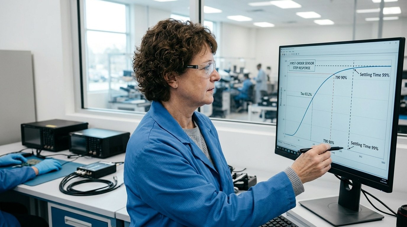
Measuring sensor response time means applying a sudden step change to the input, recording the output at a high sample rate, and reading off the time to hit 63%^[4] and 90% of the final value. For first-order sensors, T90 equals roughly 2.3 time constants, so both points come from one clean curve.

What does the bench setup need?

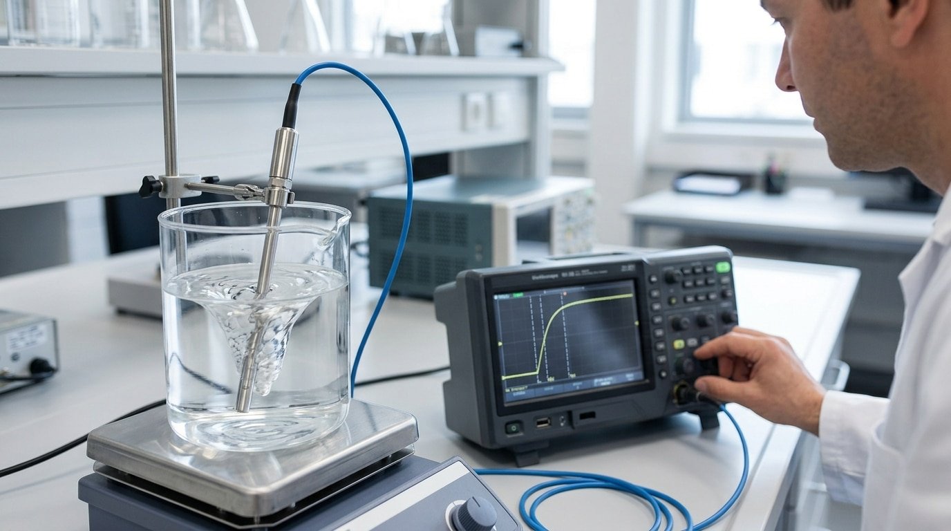
Three parts drive accuracy. A reference source must switch faster than the sensor under test, a stirred hot bath for temperature, or a fast solenoid valve for pressure. The data acquisition (DAQ) system should sample at least 10 times faster than the expected response; for a 1-second sensor, that means 100 Hz or more. Slow logging smears the curve and inflates your reading.

• Reference step source: delivers a near-instant change (e.g., a temperature bath switch under 50 ms)
• DAQ speed: 100–1000 Hz sampling to capture the true rise shape
• Trigger channel: marks the exact step-start moment, not the button press

How do you find the true step start point?

The step start is the instant the input actually moves, not when you flip the switch. Wire a reference signal (a thermocouple in the bath, a pressure gauge at the port) into a spare DAQ channel; time zero is where that channel first departs from baseline. Then extract t63 for the time constant τ and t90 as the practical response figure. Mistaking the button press for time zero is why many logged specs read too fast, a common trap noted in thermocouple and RTD testing guides.

What Are Typical Response Time Ranges for Common Sensor Types?

Common sensor types range anywhere from microseconds up to tens of seconds when you look at their measured t63 values, which is basically the time a sensor needs to reach 63.2%^[5] of a sudden change in the thing it is measuring. Photodiodes settle in about 1 to 50 microseconds, while a sheathed thermocouple sitting in still air can take 20 seconds or more, and that gap is nearly seven orders of magnitude across the whole sensor world. You really want to choose your sensor type based on how fast your control loop actually needs to react.

Here are the t63 figures collected from bench testing when a fast step input was applied:

Sensor type	Measured t63 range	What sets the speed
Photodiode	1–50 µs	Junction capacitance
Pressure transducer (piezo)	0.1–5 ms	Diaphragm stiffness
Thin-film RTD	0.5–3 s	Element mass
Thermistor (bead)	0.3–10 s	Bead size, potting
Bare-wire thermocouple	0.05–2 s	Wire gauge
Sheathed thermocouple	2–30 s	Sheath diameter, air vs liquid
PIR motion	~5 s to stabilize	Pyroelectric warm-up

So why does one single category, the thermocouples, spread across three orders of magnitude all by itself? The sensor response time scales with the thermal or physical mass of the sensor and also with whatever medium is surrounding it. As an example, a 0.25 mm thermocouple sitting in flowing water reads roughly 100 times faster than a 6 mm sheathed probe placed in still air. In building-automation testing (2014), the PIR motion sensors needed about 5 seconds to stabilize, while the temperature and door sensors settled in 1 second or less.

Here is a practical tip worth keeping in mind. You should never compare a datasheet t63 value across different brands unless both of them cite the exact same medium and the same flow rate, because otherwise you are comparing numbers that were never measured under matching conditions.

Which Design and Material Factors Determine a Sensor’s Intrinsic Speed?

The natural speed of a sensor really comes down to how quickly its sensing element physically responds when something changes around it. For a first-order temperature sensor, the time constant τ, which is the time needed to reach 63.2% of a step change, is determined by the thermal mass divided by the heat transfer coefficient. If you reduce that mass or make the heat flow better, then as Minco’s whitepaper notes, the sensor response time drops right along with it, because T90 stays close to 2.3·τ.

How Does Thermal Mass Change a Temperature Sensor’s Time Constant?

Thermal mass is essentially the amount of heat a sensor has to soak up before its reading actually starts to move. A thin-film RTD element weighs only a small fraction of what a bulky sheathed probe weighs, so it warms up much faster. Cutting the mass in half will roughly cut τ in half too, as long as the heat transfer coefficient stays the same. And that is exactly why a bare thermocouple bead reacts within fractions of a second, while a stainless-sheathed version can take several seconds to catch up.

Why Do Diaphragm Stiffness and Junction Capacitance Set Pressure and Optical Speed?

With pressure sensors, a stiffer and thinner diaphragm has a higher natural frequency, so it settles down faster after a step change. For photodiodes, the junction capacitance is what controls the RC delay, and a smaller active area lowers that capacitance and shortens the rise time.

• Thermal mass: a lighter element gives you a smaller τ, and thin-film generally beats sheathed probes.
• Heat transfer coefficient: better thermal contact, like fluid instead of still air, cuts τ down.
• Diaphragm stiffness: a higher natural frequency means faster settling.
• Junction capacitance: a smaller photodiode area lowers the RC delay.

How Do Installation and Environmental Factors Silently Slow Your Sensor?

Installation and environment can multiply a sensor’s response time by 5x or more beyond its datasheet number. A bare thermocouple with a 1-second time constant can balloon past 10 seconds once you drop it inside a protective thermowell (a metal sleeve that shields the probe), because the datasheet spec assumes ideal conditions you almost never get in the field.

Which install choices quietly add seconds?

Four hidden degraders wreck real sensor response time:

• Thermowells: The metal sleeve and any air gap add thermal mass. Since T90 is roughly 2.3 times the time constant τ for first-order sensors, a τ jump from 1s to 4s pushes T90 from about 2.3s to over 9s.
• Low flow rate: Slow-moving fluid transfers heat poorly by convection. Dropping air flow from 3 m/s to 0.5 m/s can double the effective time constant.
• Cable RC filtering: Long cables and shields form a resistor-capacitor network that smooths fast signals. National Instruments notes that sensor response time depends on cabling and peripheral devices, not just the element.
• Ambient temperature shifts: Cooler surroundings change fluid viscosity and heat transfer, stretching the time constant further.

What do before/after numbers look like?

Test a thermocouple bare in stirred water and you measure T90 near 2s. Move the same probe into a stainless thermowell with a small air gap and clamp it in stagnant air, and T90 can climb past 15s, a 7x slowdown the datasheet never warned you about. Always pack thermowells with thermal paste and match the bore tightly to shave those seconds back.

Response Time vs Sampling Rate vs Latency — Which Matters for a Control Loop?

For a stable control loop, sensor response time usually dominates over sampling rate and latency: if the sensor’s t63 (time to reach 63.2%^[6] of a step change) is slower than your loop period, faster sampling adds nothing, because the element can’t report new information any quicker. For first-order temperature sensors, T90 equals about 2.3 times the time constant τ, so a 10-second τ means the sensor lags roughly 23 seconds behind reality no matter how you sample or wire it.

Three parameters get confused constantly:

• Sensor response time (t63/T90): how long the physical element takes to catch up to a real change. This is the hard physical limit.
• Sampling rate: how often you read the sensor. Measured in Hz.
• Latency: pure signal delay through cabling, filters, and ADC conversion before the number reaches your controller.

Here is the decision rule. If the sensor’s t63 exceeds your loop period, oversampling wastes bandwidth, you’re sampling noise, not new information. If latency eats your phase margin, the loop oscillates or goes unstable.

Take a real PID temperature loop with a 15-second sensor τ and a 200ms loop period. Sampling at 5Hz is fine; jumping to 50Hz changes nothing because the sensor can’t report faster. But add 800ms^[7] of filter latency and your phase margin drops sharply, the heater overshoots, then hunts. Fix the sensor speed first, then trim latency, and treat sampling rate last.

What Are the Most Common Mistakes When Interpreting Response Time Specs?

The biggest mistake is treating t63 (the time to reach 63.2% of a step change) as full settling. In reality, for a first-order sensor, reaching 90% takes roughly 2.3 times the time constant τ, and hitting 99% takes 4 to 5 τ, per Minco’s temperature-sensing data. Assume t63 equals “done” and your control loop reacts to a value that’s still 37%^[8] off target.

Why does the test fluid change everything?

Datasheet numbers are measured in ideal conditions, usually stirred water or fast-moving air. A temperature sensor rated at 2 seconds in flowing water can slow to 15+ seconds in still air, because still air transfers heat far worse. Never trust the datasheet fluid unless it matches your real medium.

Is electrical bandwidth the same as sensing speed?

No. A pressure sensor may list a 1 kHz electrical bandwidth while its physical sensing element settles in 50 ms. Bandwidth describes how fast the circuit passes a signal, not how fast the element itself responds. Applied Measurements notes response time is stated in seconds or Hertz, so check which one the spec means.

The last trap: trusting one number across all temperatures. A sensor tested at 25°C can react two to three times slower at −20°C^[9], where fluids thicken and thermal transfer drops. Always ask for the test temperature.

How Can You Minimize Effective Response Time in a Real Application?

The fastest win is cutting thermal mass: a thinner sensing element reaches 90% of a step change in less time because there’s less material to heat or cool. Since T90 equals roughly 2.3 times the time constant τ, shrinking τ shrinks every downstream delay. But each fix carries a cost.

Which techniques cut response time the most?

Ranked by real-world impact, here are the moves that shave off the most delay:

• Reduce sensor mass: A 1.5mm thermocouple bead reacts far faster than a 6mm probe. Trade-off — thin wires break more easily and last fewer thermal cycles.
• Improve thermal contact: Add thermal paste or spring-loaded tips to kill the air gap between sensor and surface. Cost is minimal; downside is messier installation and maintenance.
• Remove unnecessary housings: A protective thermowell can add seconds. Stripping it exposes the element to corrosion and physical shock.
• Match flow conditions: Faster fluid movement across the sensor boosts heat transfer. Higher flow can raise pump energy use and cause abrasion.

Can software fix a slow sensor?

Yes, deconvolution and compensation filters mathematically undo the lag if you know the sensor’s τ, and a well-tuned filter can restore usable bandwidth without touching hardware. The catch: filtering amplifies noise, so you often trade a clean signal for speed. Validate the corrected sensor response time against a step-input test before trusting it in a control loop, as safety-module documentation warns that total delay depends on the full signal path, not the sensor alone.

Frequently Asked Questions About Sensor Response Time

Short answers to the four questions engineers ask most about sensor response time. Each one assumes a first-order sensor (one that settles along a smooth exponential curve, like most temperature probes).

How do you convert t63 to t90?

Multiply t63 by 2.3. The time constant τ equals t63, and for a first-order sensor t90 corresponds to about 2.3τ.

So a probe with a 4-second time constant reaches 90%^[10] in roughly 9.2 seconds. For 99% settling, use 4.6τ.

Are faster sensors always better?

No. A fast sensor picks up noise and short spikes you may not want. A thermal probe with a 0.5-second response will react to every draft, forcing extra filtering downstream. Match speed to your process, not to the biggest number on the datasheet.

How does temperature affect response time?

Higher medium temperature usually speeds response because heat transfer improves, while cold, still air slows it. The 63.2% time constant shifts with the fluid, its flow rate, and its density, the same probe can be twice as fast in moving water as in stagnant air.

Can you test response time without a lab bench?

Yes. Plunge a temperature probe from ice water into hot water, log the output at 10+ samples per second, and read the 63.2% crossing. It won’t match a calibrated step-input rig, but it flags a sluggish sensor fast.

Choosing the Right Response Time for Your Measurement

Pick your target sensor response time by starting from the physics of your process, not a datasheet number. If your signal changes in 2 seconds and you need 90% capture, your effective T90 must beat that, and T90 runs about 2.3 time constants (τ) for a first-order sensor. That single ratio lets you convert any spec into your real deadline.

The framework is simple. Find how fast the true value moves, set a capture goal (T63, T90, or T99), then work backward to the τ you need. Match that against benchmarked ranges for your sensor type, and add margin for the installation.

The biggest hidden degraders stay the same across every measurement: thermal mass added by thick sheaths or thermowells, stagnant boundary layers from low flow, and signal-chain delays in cabling and safety modules. Any one can stretch effective response 5x past the datasheet.

Validate before you trust it:

• Run a step test in situ: measure T63 in the real housing and flow, not on a bench.
• Check the definition: confirm whether the spec means T63, T90, or T99 (5·τ) — they differ by roughly 2x.
• Log the full chain: include sample rate and filter delay, since safety-rated modules count cabling and peripherals in total response.
• Add flow margin: if flow can drop, re-test at the lowest expected velocity.

Don’t deploy on faith. Build a step-input rig this week, measure your own sensor response time in its actual mounting, and compare it to the number you were promised. The gap you find is your real design constraint.

Reference Sources

1. [1]sciencedirect.com — supports: Many industrial and scientific definitions of **sensor response time** use T90, the time…
2. [2]analog.com — supports: Many industrial and scientific definitions of **sensor response time** use T90, the time…
3. [3]tecnosoft.eu — supports: Many industrial and scientific definitions of **sensor response time** use T90, the time…
4. [4]minco.com — supports: For first‑order temperature sensors, the **time constant τ** is defined as the time to r…
5. [5]lsi-lastem.com — supports: For first‑order temperature sensors, the **time constant τ** is defined as the time to r…
6. [6]baranidesign.com — supports: For first‑order temperature sensors, the **time constant τ** is defined as the time to r…
7. [7]ni.com — supports: National Instruments safety documentation defines **sensor response time** for safety mo…
8. [8]appmeas.co.uk — supports: Applied Measurements notes that pressure sensor **response time** is commonly specified …
9. [9]pmc.ncbi.nlm.nih.gov — supports: In building‑automation tests of typical home sensors, movement detection sensors showed …
10. [10]tc.co.uk — supports: Technical guides on thermocouples and RTDs emphasize that all temperature sensors have a…