What is sensor repeatability and how is it measured

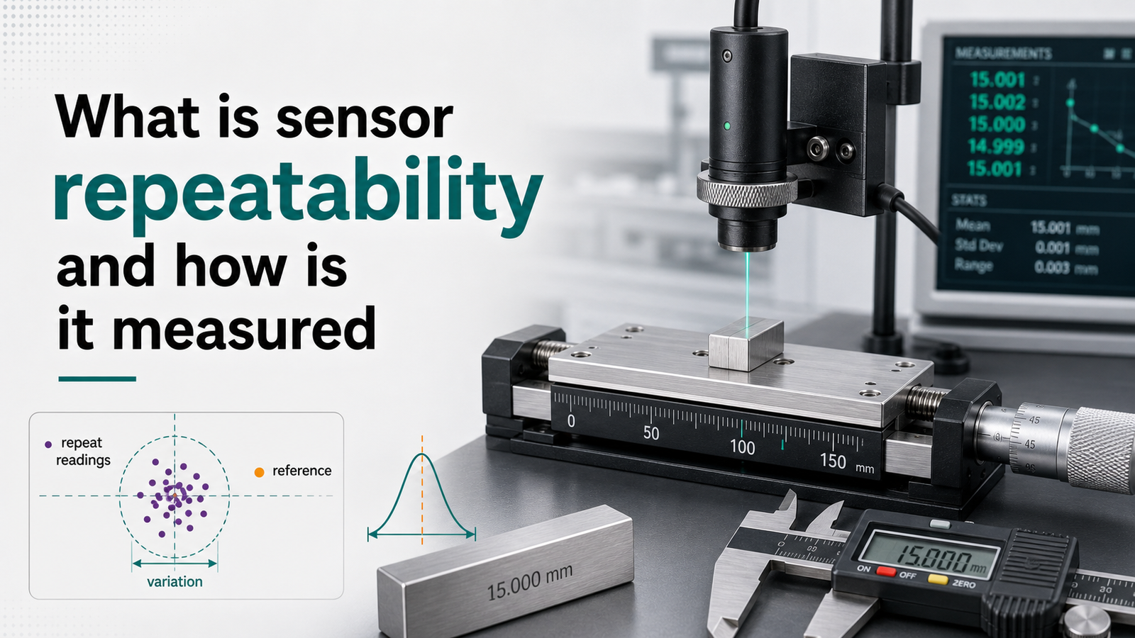
Sensor repeatability is the largest difference between transducer output readings when the same load is applied repeatedly under identical loading and environmental conditions. Expressed as a standard deviation or percentage of full scale (FS), it measures how tightly readings group—not their closeness to the true value. Precision load cells achieve 0.02–approximately 0.05%^[1] FS repeatability, while industrial sensors typically range from 0.1–approximately 0.5% FS. For example, applying the same input ten times reveals how consistently those ten readings cluster together.

This guide sets out to answer the questions engineers really do search for. How does repeatability actually differ from accuracy and hysteresis? What test procedure is used to measure it? Which formula turns raw readings into a repeatability number that means something? And what specifications should you insist on when you’re choosing a sensor?

Quick Takeaways

• Repeatability measures reading spread under identical repeated inputs, not accuracy to true value.
• Precision load cells achieve 0.02–approximately 0.05% FS; industrial sensors typically hit 0.1–0.5% FS.
• Calculate repeatability as standard deviation across three or more cycles at same load.
• A sensor can repeat tightly yet read consistently wrong—repeatability isn’t accuracy.
• Control temperature, mounting torque, and cable strain to prevent repeatability degradation.

What’s sensor repeatability?

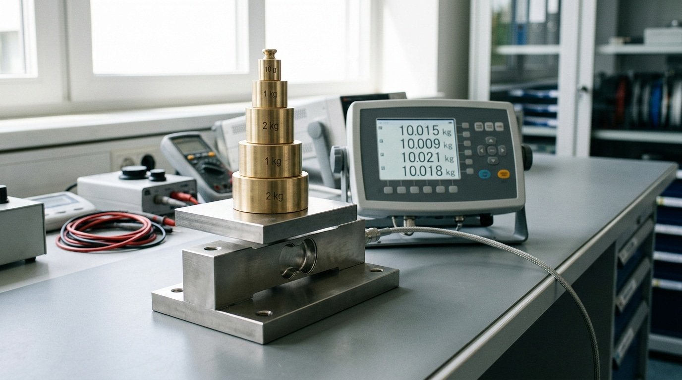
Sensor repeatability is basically the spread of output values you get when the same input gets applied again and again under identical conditions. Say you press a load cell with exactly 10 kg five separate times and you read back 10.02, 9.98, 10.01, 9.99, and 10.00 kg.

That scatter you see is the repeatability. It answers one simple question, which is how consistent a sensor is against itself, rather than how close it actually lands to the true value.

Since repeatability really describes the sensor’s fight with its own noise, a sensor can read 2%^[2] off the real number every single time and still be highly repeatable, because the readings all agree with each other. That is exactly why repeatability values always need to be smaller than accuracy values on a datasheet, as LMI Technologies points out for their 3D measurement sensors.

Engineers tend to express repeatability in three common ways:

• Percentage of full scale (±%FS): this is the spread shown as a fraction of the sensor’s total range. Some pressure sensors carry a repeatability index of 0.075% FS or even better than that.
• ±3σ (three standard deviations): a statistical band that covers roughly 99.7% of the repeated readings.
• Engineering units: these are raw values like ±0.01 mm or ±5 µV, which come in handy when the %FS figure hides the real magnitude of the number.

The vocabulary here comes straight from formal standards. The ISA and the JCGM/VIM (International Vocabulary of Metrology) define repeatability as measurement precision under a fixed set of conditions, meaning the same operator, the same instrument, the same location, all over a short window of time. Reproducibility, by contrast, actually lets those conditions change. Confusing the two leads you right into wrong sensor picks, a trap that gets covered in later sections.

How is repeatability different from accuracy, precision, resolution and hysteresis?

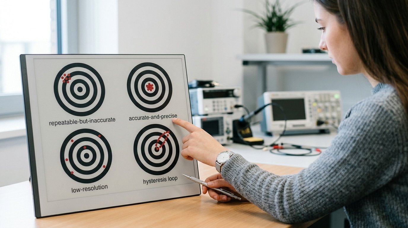
Repeatability measures how much the same sensor’s output varies when you apply the identical input again and again; accuracy measures how close those readings sit to the true value. A sensor can be repeatable but inaccurate, or accurate on average yet scattered. These are separate specs, each derived from the same raw data differently, the example below pulls all five from one dataset.

Picture one pressure sensor read 10 times at a true 100.0 kPa reference. The readings: 101.2, 101.1, 101.3, 101.2, 101.1, 101.2, 101.3, 101.1, 101.2, 101.2 kPa.

Watch how each spec falls out of that single dataset.

• Repeatability: the spread of those repeated readings — here a standard deviation of about 0.07 kPa. Tight scatter, so sensor repeatability is excellent.
• Accuracy: distance from truth. The mean is 101.19 kPa^[3] versus a real 100.0 kPa — a 1.19% error. Repeatable, but off.
• Precision: closeness of readings to each other, essentially the same as repeatability here — high.
• Resolution: the smallest change the sensor can report, say 0.1 kPa. By definition, repeatability can be no better than resolution.
• Hysteresis: the output gap when you reach 100 kPa rising versus falling — invisible in one-direction data, so it needs a separate up-and-down sweep.

The takeaway: a 1.19% bias is fixable with calibration; a wide standard deviation isn’t. That is why engineers prize a low repeatability index, under 0.075% FS on quality pressure sensors, over headline accuracy.

How do you calculate repeatability from repeated measurement data?

Take 10 readings at one fixed setpoint, compute the mean and standard deviation (a measure of how spread out the numbers are), then report ±3σ as a percentage of full scale. Zimmer & Peacock notes that sensor repeatability is quantified by the standard deviation of repeated trials of the same quantity under identical conditions. This band tells you the worst-case spread you can trust.

Here is a worked example. A pressure sensor with 100 kPa full scale is loaded to 50 kPa^[4] ten times.

The readings (kPa): 50.02, 49.98, 50.05, 49.97, 50.01, 50.03, 49.99, 50.04, 49.96, 50.00.

• Mean (average): sum all readings ÷ 10 = 500.05 ÷ 10 = 50.005 kPa
• Standard deviation (σ): subtract the mean from each reading, square it, average those squares, take the square root = 0.0296 kPa
• ±3σ band: 3 × 0.0296 = ±0.089 kPa (covers 99.7% of readings)
• Convert to %FS: 0.089 ÷ 100 × 100 = 0.089% FS

So this unit’s repeatability is 0.089% FS. Use the sample standard deviation formula (divide by n−1, not n) in Excel with =STDEV.S(range).

Ten readings is a bare minimum; 30+ trials give a more stable σ. Compare your 0.089%^[5] against datasheet claims like 0.075% FS to judge if the part meets spec.

How is sensor repeatability tested in practice?

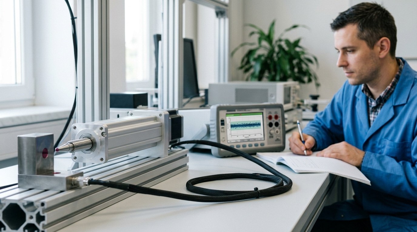
Sensor repeatability gets tested by driving the sensor to the same setpoint many times from the same direction, then recording how much the output readings spread out under conditions that stay fixed. A typical procedure takes 10 to 30 approaches per point and expresses the result either as a standard deviation or as a percentage of full scale (FS). This tells you how tightly the sensor tracks against itself before you trust it inside a control loop.

Run the test correctly and small numbers actually become believable. First, cycle the sensor across its full range to normalize its thermal and mechanical state. Then approach each setpoint, wait for a settling time that stays fixed, and log the reading. Uncontrolled settling is generally the most common way engineers accidentally inflate their own repeatability figures, since a reading logged before the output has stabilized adds scatter that really belongs to the timing rather than the sensor.

What’s the difference between unidirectional and bidirectional tests?

Unidirectional repeatability measures moves to a point that always arrive from the same prior position, while bidirectional adds moves from random or opposite prior positions, which folds in hysteresis effects that Xeryon documents for positioning stages. Bidirectional numbers are always going to be larger. And if a datasheet doesn’t state the direction, you should treat the figure as optimistic.

How does sample size affect confidence?

More samples tighten up your estimate. With only 5 readings, your standard deviation could be off by a wide margin, and the NIST guidance on measurement uncertainty shows why 20 to 30 trials give you a stable estimate. You really should report the sample count alongside the spread, otherwise the number means very little on its own.

How do you compare repeatability figures across different manufacturers’ datasheets?

You can’t compare them directly. A “±0.1% FS” figure, a “±0.05% reading” figure, and a “3σ” figure use three different math bases, so the numbers mean different things. Convert all three to the same basis first: standard deviation (1σ) as a percentage of full scale (FS). Only then does the smaller number actually win.

💡 Counterintuitive: A sensor with excellent 0.02% FS repeatability can still read consistently wrong. Repeatability only measures how tightly ten repeated readings cluster—not their closeness to the true value. Evidence: a load cell can return the same offset reading every cycle while carrying a systematic error from poor calibration. Tight grouping proves consistency, not accuracy; verify both by calibrating against a known reference, not just repeat-testing.

Two traps hide inside datasheet numbers. First, % FS vs % reading: a % FS spec is fixed across the range, while a % reading spec shrinks with the measured value.

At 20% of range, a “±0.05% reading” sensor is only spending 0.05%^[6] of a small number,much tighter than it looks at full scale. Second, σ multiplier: a “3σ” claim already includes 99.7% of the spread, so it’s roughly 3× wider than a bare “±” figure that may quietly be 1σ.

Normalize like this: divide any 3σ value by 3 to get 1σ, and restate % reading at your actual operating point before comparing.

Vendor	Datasheet claim	Basis	Normalized 1σ (%FS)
A	±0.10% FS	1σ, full scale	0.100%
B	±0.05% reading @ 40% range	1σ, of reading	0.020%[7]
C	±0.18% FS (3σ)	3σ, full scale	0.060%

After normalizing, Vendor B wins at that operating point,not the one with the smallest raw digits. This is why FUTEK expresses sensor repeatability as a standard deviation or a percentage of full scale: without a stated basis, the number is meaningless.

What environmental and operational factors degrade repeatability?

Temperature drift, short warm-up, mounting stress, supply-voltage swings, and aging all eat into sensor repeatability. Temperature is usually the biggest offender, often shifting output by 0.01,0.05% of full scale per degree Celsius. Some of these you can remove through calibration; others set a hard floor no math can undo.

Which factors can calibration remove, and which are permanent?

Calibration removes predictable, repeatable errors. It can’t remove random noise. Here is how the main factors split:

Factor	Typical magnitude	Removable by calibration?
Temperature drift	0.01–0.05% FS / °C	Yes — if temperature is measured
Insufficient warm-up	0.05–0.2% FS in first 15–30 min	No — just wait for stability
Mounting stress	0.02–0.1% FS	Partly — re-zero after mounting
Supply-voltage variation	0.005–0.02%[8] FS / V	Yes — with ratiometric wiring
Long-term aging	0.1–0.25% FS per year	No — sets a hard floor

Warm-up matters more than people think. A load cell or pressure sensor needs 15 to 30 minutes to reach thermal equilibrium. Skip it and your repeatability trials will drift as the electronics heat up. This is why the definition ties repeatability to identical loading and environmental conditions, change the conditions and you no longer measure repeatability at all.

Mounting stress is sneaky: over-torquing bolts on a strain gauge sensor bends the flexure and shifts the zero, which is why re-zeroing after mounting only partly recovers it. Random noise and aging, unlike temperature or supply-voltage effects, can’t be calibrated away, they define the best your sensor will ever do.

What repeatability mistakes cause bad sensor decisions?

The most costly repeatability mistake is assuming that a highly accurate sensor is also repeatable. It isn’t the same thing. A sensor can hit the true value on average yet scatter widely on repeated tries. By definition, repeatability must be smaller than accuracy in a spec, so a datasheet listing only accuracy tells you nothing about run-to-run consistency.

Four errors trip up engineers again and again:

• Trusting accuracy as a proxy: A ±0.5% accurate sensor may still drift ±0.3% between identical readings. Your control loop feels the scatter, not the average.
• Ignoring the sigma multiplier: A “±0.02% FS” figure could be 1σ (68% of readings) or 3σ (99.7%). Reading a 1σ number as a worst-case guarantee understates real spread by 3×.
• Testing at one point only: Repeatability often worsens near the range extremes. Checking only mid-scale hides the point where your process actually operates.
• Skipping warm-up: Cold sensors drift as internal temperature stabilizes. A reading taken 2 minutes after power-on can wander more than one taken after the 30-minute soak the datasheet assumed.

Each mistake shows up in production as false rejects, phantom process shifts, or a control loop that hunts. A pressure sensor rated at ≤0.075% FS repeatability only delivers that number under the conditions it was measured. Test the way you’ll actually use it, same setpoint you run daily, after full warm-up, and confirm which sigma the vendor quoted before you trust any sensor repeatability figure.

How do you use repeatability specs when selecting a sensor for a project?

Match the repeatability budget to what your application actually needs. A rough rule: your sensor repeatability should be 4,10 times tighter than your smallest acceptable output change. For closed-loop control targeting ±0.5°C^[9], pick a sensor with repeatability under ±0.1°C. Anything looser and your controller will chase noise instead of the real signal.

Use this if-then guide to set the target:

• Closed-loop control: Need repeatability 5–10× better than your control tolerance. Poor repeatability here shows up as hunting or limit-cycle oscillation around the setpoint.
• Go/no-go gauging: Repeatability must be under one-tenth of your pass/fail gap. Miss this and good parts get rejected while bad ones slip through.
• Trend monitoring: Repeatability matters less than long-term drift. Prioritize a low drift spec instead.

Split a total error budget across three parts. A common allocation for a precision instrument: repeatability 40%, resolution 20%, drift 40%. Keep resolution finer than repeatability, since University of Pisa mechatronics material notes repeatability can be, at best, only as good as the sensor’s resolution. A sensor with 0.01% resolution but 0.075% FS repeatability is limited by repeatability, not the display digits.

One practical trap: buy a bit of margin. If your budget allows ±0.05%^[10] FS, target a sensor rated ±0.03% FS. Datasheet numbers degrade with real mounting stress and warm-up, so the extra headroom keeps you inside spec in the field.

Frequently asked questions about sensor repeatability

Short answers to the questions engineers ask most before trusting a repeatability number. Each one covers a real trap that trips up sensor selection.

Can repeatability be better than resolution?

No. Repeatability can be at best as good as the resolution of the sensor, according to mechatronics teaching material from the University of Pisa. Resolution is the smallest change the sensor can report. You can’t repeat within a step you can’t detect. If a datasheet claims repeatability finer than resolution, treat it as a marketing error.

How many trials are enough?

Run at least 30 readings at one fixed setpoint. Below 10, your standard deviation estimate swings wildly and can under-report the true spread by half. For critical process control, use 50 to 100 cycles so the sample captures slow drift and occasional outliers.

Does calibration improve repeatability?

Rarely. Calibration corrects systematic offset and slope, which fixes accuracy. It doesn’t shrink the random scatter that defines sensor repeatability. A poorly repeatable sensor stays scattered after calibration,you just center the scatter on the true value.

How does repeatability relate to reproducibility?

Repeatability holds every condition constant. Reproducibility deliberately changes operators, days, or instruments, then measures variation. Repeatability is always the smaller, more optimistic number.

Key takeaways for evaluating sensor repeatability

Evaluating sensor repeatability comes down to four steps: pull the datasheet number, normalize it to a common basis, express it as ±3σ in percent of full scale (%FS), then check it against your application’s error budget. Do this before you buy, not after the sensor fails a repeat-loading test on your bench.

The trap is that datasheet figures rarely share a basis. One vendor quotes ±1σ, another quotes peak-to-peak span, a third gives %FS at a single setpoint. Since repeatability must be smaller than accuracy by definition, a suspiciously tiny number often signals a narrow test condition, not a better sensor.

Run the math yourself. Convert every candidate to the same statistic and the same reference before comparing.

• Extract: find the raw figure and its stated basis (σ, ±3σ, or peak span).
• Normalize: multiply single-σ specs by 3 to reach a 99.7% coverage band.
• Convert to %FS: divide by the full-scale range so 0.075%FS on a 100-bar sensor equals 75 mbar.
• Match the budget: repeatability should consume no more than one-third of your total allowed error.

A pressure sensor rated at 0.075%FS repeatability leaves headroom for a process needing 0.5% total accuracy. One rated at 0.3% eats most of that budget alone. Plug your candidates into this workflow, and sensor repeatability stops being a marketing number and becomes a purchasing decision you can defend.

Reference Sources

1. [1]futek.com — supports: FUTEK defines **sensor repeatability** as the maximum difference between transducer outp…
2. [2]zimmerpeacock.com — supports: Zimmer & Peacock states that **sensor repeatability** is quantified by calculating the s…
3. [3]lmi3d.com — supports: LMI Technologies defines **repeatability** in inline 3D measurement sensors as the varia…
4. [4]apogeeinstruments.com — supports: Apogee Instruments explains that **sensor repeatability** describes how consistent a par…
5. [5]yokogawa.com — supports: Yokogawa states in its technical information that **sensor repeatability** is the abilit…
6. [6]microsensorcorp.com — supports: Microsensor Corp specifies that for its pressure sensors, the **repeatability index** is…
7. [7]xeryon.com — supports: Xeryon defines **unidirectional repeatability** of positioning stages as the standard de…
8. [8]rheonics.com — supports: Rheonics describes measurement-device **repeatability** as the ability of a sensor to pr…
9. [9]sense-the-world.com — supports: Sense-the-World explains that in proximity sensors, **repeatability** (repeat positionin…
10. [10]didawiki.cli.di.unipi.it — supports: Basic mechatronics teaching material from the University of Pisa defines **sensor repeat…