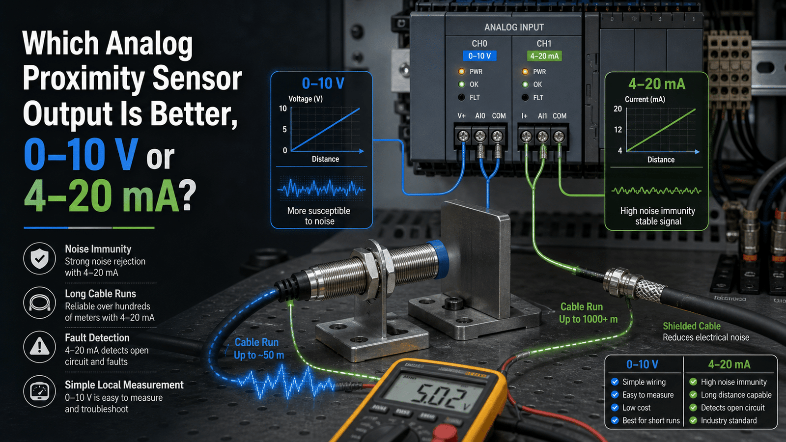
An analog proximity sensor 0-10V 4-20mA outputs a variable signal proportional to target distance, with 4–20mA best for long cable runs and noisy environments and 0–10V best for short runs and low-cost setups. The 4–20mA current loop holds accuracy over 100+ meters and detects broken wires (0mA signals a fault), while 0–10V is cheaper and reads directly on most voltage-input PLC cards but loses accuracy from cable resistance and electrical noise.
And why does the 4,20mA signal hold up against electrical noise so much better than the alternative?
There’s also the question of when 0,10V is still the smarter thing to buy. And which of the two options fits your PLC and your wiring budget best?
Quick Takeaways
- Choose 4–20mA for cable runs over 100 meters or noisy environments.
- Pick 0–10V for short runs and low-cost, budget-conscious setups.
- Use 4–20mA fault detection: 0mA flags broken wires instantly.
- Verify your PLC input card matches voltage or current signals.
- Buy selectable sensors to switch between 0–10V, 4–20mA, and 0–20mA modes.
What does an analog proximity sensor with 0–10 V or 4–20 mA output actually do?
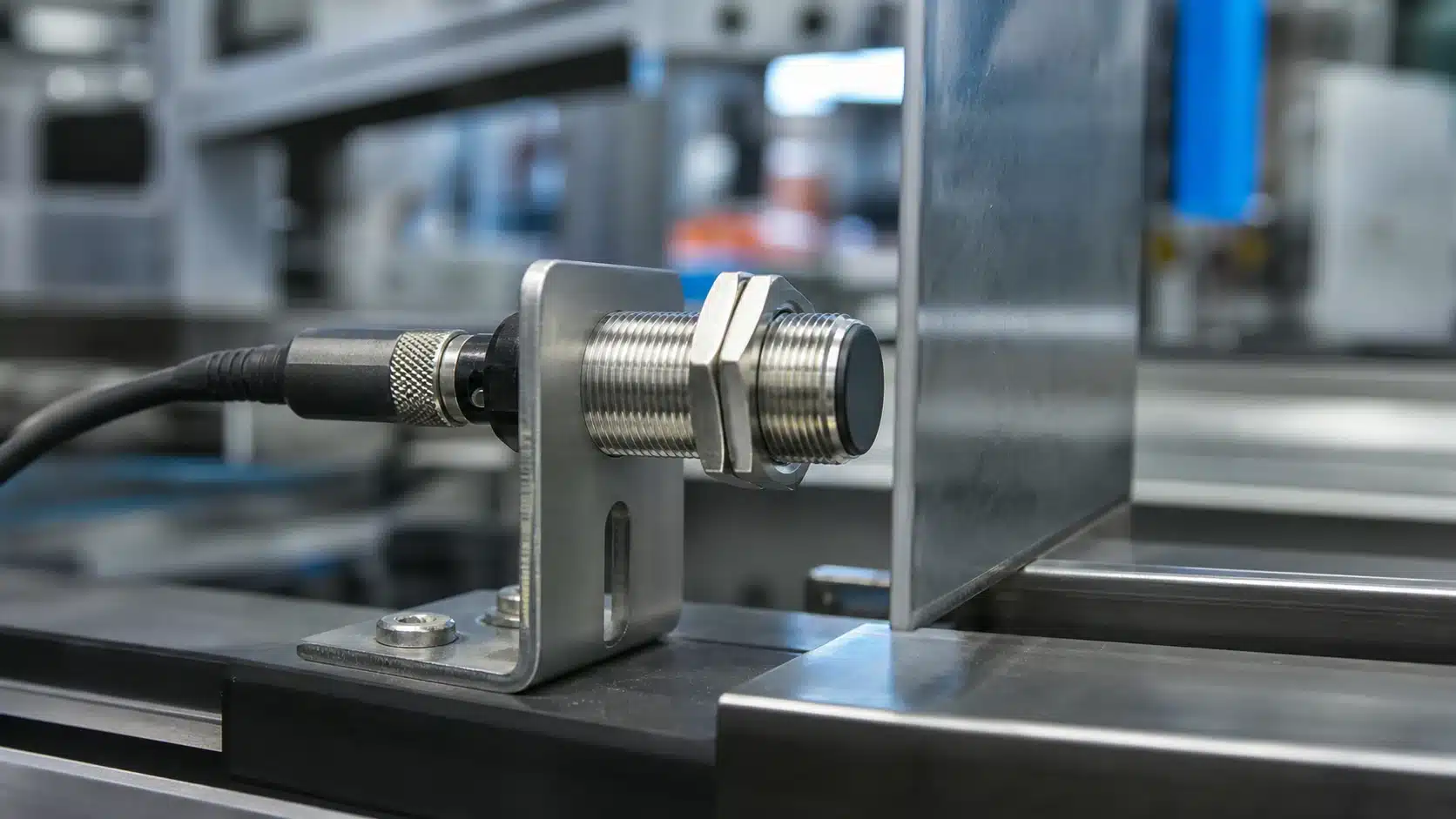
An analog proximity sensor 0-10V 4-20mA sends out a signal that goes up and down depending on exactly how far away a metal target sits, rather than simply switching on or off. A regular switching sensor really answers just one question, which is whether metal is present, yes or no. The analog kind answers something trickier, which is how far away the metal is at this very moment. As the target gets closer, the output rises right along with it, so if you move it 2 mm the current changes by a set amount for every millimeter, and your PLC reads that number and does something with it.
One M12 flush model reads a 0.1,3 mm detection window with 0.02 mm repeat accuracy (2026), which means a controller actually sees position rather than just whether something is there. That lets you measure gaps instead of only counting objects.
Four jobs come up over and over out on the plant floor:
- Fill-level control: The sensor follows a rising surface and keeps it inside a tight band, which cuts down on overfill waste.
- Roll diameter: When a paper or film roll unwinds, the shrinking diameter changes what the sensor reads, so the drive adjusts its speed to hold the tension steady.
- Part positioning: A stamping cell confirms that a blank is sitting within a 0.5 mm tolerance before the press comes down.
- Web tension monitoring: The position of a dancer arm feeds back a continuous distance value, letting the line correct any sag as it happens.
The 4,20 mA version brings along a built-in fault check that professionals count on. A reading of 0 mA tells you a wire is broken, not that you have a valid “zero distance.” That live-zero trick is basically why current output wins out on long, noisy cable runs, which happens to be the topic of the next section.
What are the key differences between 0–10 V and 4–20 mA outputs?
The core difference is what the signal carries: 0,10 V sends a voltage, while 4,20 mA sends a current. Current wins on noise immunity and long cable runs; voltage wins on receiver simplicity and cost. For an analog proximity sensor 0-10V 4-20mA, this single choice affects wiring, distance, and fault detection.
Current loops resist electromagnetic interference (EMI), stray electrical noise from motors or drives, because the same current stays constant along the whole wire. Voltage signals drop as cable length grows, since wire resistance eats into the reading.
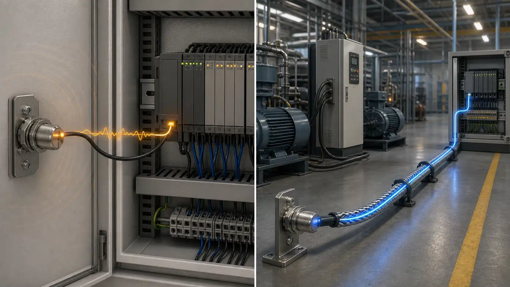
The biggest practical edge is live-zero detection. A 4,20 mA loop never reads 0 mA when healthy, so if the receiver sees 0 mA, the wire is broken or the sensor died. A 0,10 V signal reading 0 V looks identical to a real “sensor at zero distance”, you can’t tell a fault from a valid low reading.
| Spec | 0–10 V | 4–20 mA |
|---|---|---|
| Signal type | Voltage | Current |
| EMI immunity | Lower | Higher |
| Wire-break detection | No | Yes (0 mA = fault) |
| Typical load limit | ≤2 kΩ | 400Ω max |
| Receiver cost | Lower | Slightly higher |
These 2026 load figures come from a real M12 flush sensor spec listing 15,30 VDC operating voltage. Notice the current loop tolerates far less resistance, plan your wiring accordingly.
Which output is better for long cable runs and noisy environments?
When you are dealing with long cable runs and factories full of electrical noise, the 4,20 mA option really comes out ahead. A current loop keeps its accuracy across hundreds of meters and simply ignores the electromagnetic interference (EMI) that comes off variable frequency drives (VFDs) and motors. A 0,10 V signal, on the other hand, starts to lose accuracy once you get past about 10,30 m, because the resistance in the wire pulls the voltage down and the noise picked up along the way corrupts the reading.
The reason for this is basically simple physics. In a current loop, the very same milliamps travel through every point along the wire no matter how long that wire happens to be, so the resistance in the cable cannot change the value your PLC ends up reading. A voltage output gets no such protection, because every ohm of copper subtracts a little from the signal, and any switching noise nearby couples straight onto the wire.
What cable-length thresholds should you follow?
Try to keep 0,10 V runs under 30 m, and under 10 m when they are anywhere near VFDs or contactors. A 4,20 mA loop stays dependable out to 300 m or even more, and what mainly limits it is the load resistance budget. The KJT M12 analog sensor, for example, allows 400Ω max on current output versus ≤2K�α for voltage. That resistance ceiling is what decides how much cable plus input impedance the loop is able to carry.
How should you shield each output type?
- 4–20 mA cable: use a twisted pair with a foil shield that is grounded at one end only, on the controller side, which keeps ground-loop currents from forming.
- 0–10 V cable: a shielded twisted pair is a must here, and it should be run in its own separate conduit that stays at least 30 cm away from power lines carrying motor or VFD current.
When you are choosing an analog proximity sensor 0-10V 4-20mA model for a factory floor that has drives running, go with the current-loop version. You can save the voltage output for the short, clean wiring that stays inside a panel.
How do you choose between 0–10 V and 4–20 mA for your application?
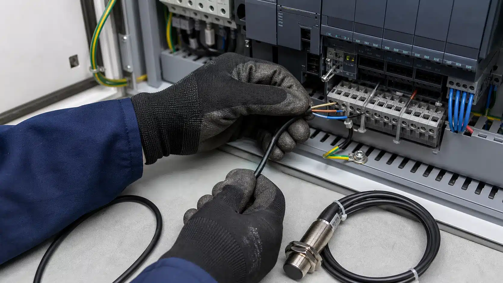
You want to match the output to your cable run, how much electrical noise is around, and the type of PLC card you’re using. If you have a short run under 10 m, a clean panel, and you’re working with a low-cost voltage input, then pick 0,10 V. But if you have a long run, motor drives sitting nearby, or you need to detect loop faults, then go with 4,20 mA. Both modes will often ship on the same analog proximity sensor 0-10V 4-20mA hardware, and you can pick between them using selectable output modes that are set by a switch.
What decision matrix should you use?
Score your particular job against five factors, and then you can read the recommended output straight off the table below.
| Factor | Favors 0–10 V | Favors 4–20 mA |
|---|---|---|
| Cable run | <10 m | >10 m |
| EMI level | Clean panel | Motor drives, VFDs, welders |
| Load resistance | ≤2 kΩ input | ≤400 Ω loop |
| PLC input card | Cheap voltage-only card | Current-capable card |
| Budget | Lowest wiring cost | Extra shielding worth it |
Those load limits are genuine design constraints, and they aren’t just loose guidelines. A typical M12 flush analog sensor caps its current output at 400 Ω max and its voltage output at ≤2 kΩ (this is the 2026 spec). And if your PLC input resistance happens to sit above 400 Ω, then the 4,20 mA loop simply can’t drive full scale, so you’ll have to switch over to voltage instead.
What if you can’t decide?
When you’re stuck, default to 4,20 mA. The current loop will tolerate wiring compromises that would completely kill a voltage signal, and switching a dual-mode sensor back to 0,10 V later on really only takes a few seconds.
How do you wire a 0–10 V or 4–20 mA sensor to sourcing vs sinking PLC inputs?
Match the sensor’s output polarity to the analog card’s input type: a sourcing sensor drives current out and pairs with a sinking card input, while a sinking sensor pulls current in and needs a sourcing card. Get this backwards and you read zero or a pinned reading. Most analog proximity sensor 0-10V 4-20mA models run on 15,30 VDC supply, so confirm your card accepts that range too.
⚠️ Common mistake: Choosing 0–10V for a 150-meter cable run to save money, then chasing “drifting” readings for weeks. This happens because cable resistance and electrical noise drop voltage signals over distance, corrupting accuracy past ~100 meters. The fix: use 4–20mA on long or noisy runs—current stays constant end-to-end, and 0mA even flags a broken wire instantly.
How do you count and connect the wires?
Wire count tells you the loop path. A 2-wire 4,20 mA sensor puts the sensor, supply, and card in series, the same current flows through everything. A 3-wire sensor adds a separate signal line, common for 0,10 V. A 4-wire sensor keeps power and signal fully independent, easiest to troubleshoot.
- Brown (V+): connects to the positive supply, 15–30 VDC.
- Blue (0 V): ties to supply common and card common (analog ground).
- Black/White (signal): feeds the card’s analog input channel.
Why do brand terminal labels cause wiring errors?
Because “AI+” on one card means signal, but “I+” on another means loop supply. One brand labels current input “mA IN,” another calls it “AI-.” Never trust the label alone, check the datasheet block diagram. For 4,20 mA, verify whether the card powers the loop (active) or expects an externally powered signal (passive). Mismatching these two burns fuses.
What load resistance limits apply to each output type?
Each output type flips the resistance rule. A 4,20 mA loop needs resistance below a maximum; a 0,10 V circuit needs input impedance above a minimum. One typical analog proximity sensor 0-10V 4-20mA spec lists a 400 Ω max load for current output and ≤2 kΩ for voltage output (2026). Exceed the current limit and the top of the range clips; drop below the voltage limit and the reading sags.
How do you calculate the maximum loop resistance for 4–20 mA?
Max loop resistance equals supply voltage minus sensor compliance, divided by 0.020 A. Say your loop runs on 24 V and the sensor needs 8 V to drive its output. That leaves 16 V for the loop. Divide 16 V by 0.020 A and you get 800 Ω total budget.
Subtract the PLC card’s input resistance, usually 250 Ω, and cable resistance. That leaves roughly 550 Ω of headroom. The 400 Ω sensor limit fits comfortably. At 20 mA the drop across 400 Ω is 8 V, well under budget.
Why does 0–10 V need high input impedance?
A voltage output can only push so much current. If the PLC input impedance is too low, current flows and the voltage droops. Most analog cards offer 10 kΩ to 1 MΩ input impedance. That easily beats the ≤2 kΩ minimum, so signal droop stays under 1%.
Verify both: check the sensor datasheet’s compliance voltage and load limit, then match against your card’s spec sheet before wiring.
How do detection range, linearity, resolution, and repeatability compare across brands?
Specs vary sharply by sensing technology, not just brand. One inductive M12 flush analog proximity sensor lists a 0.1,3 mm range, under 5% linearity, and 0.02 mm repeat accuracy in 2026. That tight window is normal for inductive metal detection, so pick the sensor family that matches your target distance first, then compare error specs.
Range differs widely. Inductive units cover short gaps; one listing shows 2,10 mm or 3,15 mm depending on configuration. An extra-distance inductive model reaches 0,4 mm. Ultrasonic and laser analog sensors extend meters, but trade off resolution.
| Type | Typical range | Linearity error | Repeatability |
|---|---|---|---|
| Inductive (M12 flush) | 0.1–3 mm | <approximately 5% | 0.02 mm |
| Inductive (extra-distance) | 0–4 mm | ~1–approximately 3% | ~0.05 mm |
| Ultrasonic analog | 50–6000 mm | ~1% | ~0.5 mm |
Output type sets your ceiling on usable resolution. An analog proximity sensor 0-10V 4-20mA feeds a 12-bit card giving 4096 steps. With 4,20 mA, only the 4,20 span carries data, so effective steps drop to about 3277. Live-zero eats resolution but flags broken wires, a fair trade for most machine builders.
What installation mistakes cause bad analog readings, and how do you avoid them?
Most bad analog readings come from five field errors: ground loops, unshielded cable near drives, wrong load resistance, mixed sourcing/sinking wiring, and no wire-break monitoring on 0,10 V. Each one leaves a fingerprint in your data. Learn the symptom, and you can trace the fault in minutes instead of hours.
Why does my analog signal drift or show a steady offset?
A steady offset usually means a ground loop. When the sensor ground and the PLC ground sit at different voltages, current flows through the shield and adds a fixed error to your voltage reading. Fix it by grounding the cable shield at one end only, the PLC side. A 4,20 mA loop resists this because current stays constant regardless of small voltage shifts, which is why an analog proximity sensor 0-10V 4-20mA setup often survives noisy plants better on the current side.
Why does the reading spike when a motor starts?
Spikes tied to motor or drive startup point to unshielded cable running parallel to power lines. Variable frequency drives radiate high-frequency noise that couples into signal wires. Keep sensor cable at least 200 mm from drive cables, cross power lines at 90°, and use twisted shielded pair. Wrong load resistance causes a different symptom: the KJT M12 analog sensor spec caps current output at 400Ω max and voltage output at ≤2kΩ; exceed those and readings clip or saturate at full scale.
Why did my broken sensor read zero instead of alarming?
A cut wire on 0,10 V reads 0 V, identical to a valid “target at minimum” signal, so no alarm fires. On 4,20 mA, a break drops current to 0 mA, well below the 4 mA live-zero, triggering an instant fault. This is why safety systems favor current loops.
Frequently asked questions about 0–10 V vs 4–20 mA proximity sensors
Buyers ask the same four questions before ordering an analog proximity sensor 0-10V 4-20mA. Below are direct answers with the specs that matter.
Can you convert between 0–10 V and 4–20 mA?
Yes. A signal converter changes one to the other for roughly $30 to $120. But skip the extra hardware when you can. Many 2026 sensors ship with selectable output modes,0-10V, 0-20mA, and 4-20mA on one part. Pick the native mode your PLC card wants. A converter adds one more failure point and a bit of extra error.
Which output is cheaper overall?
The sensor itself costs about the same. The real cost is cabling. On a run under 10 m, 0,10 V works with standard wire and is cheaper. Past 30 m, 4,20 mA saves money because you skip shielded low-resistance cable and signal boosters.
Do 3-wire and 4-wire versions differ?
Yes. A 3-wire sensor shares one line for power return and signal ground; a 4-wire keeps them separate, cutting ground-loop error. For current loops, 2-wire loop-powered types draw the 4,20 mA through the same pair that supplies power.
Is 0–10 V ever the better pick?
Yes,when your PLC has only voltage inputs, cable is short, and you need fast response with no loop settling delay. In a clean control panel with a 15-30VDC supply, 0,10 V is simple and works fine.
Choosing the right analog output — final recommendation and next steps
Default to 4,20 mA. For any industrial run over 10 m, near motors or drives, or where a fault could halt production, current wins because it survives voltage drop and rejects noise. Pick 0,10 V only for short, clean, cost-sensitive setups under 3 m with a spare voltage input card already on the PLC.
The signal type is a real decision, not a formality. Many 2026 sensors let you sidestep it entirely: one analog inductive line offers selectable 0-10V, 0-20mA, and 4-20mA modes on the same part number. If your plant mixes short benches and long cable pulls, a selectable sensor cuts your spare-parts list.
What should you confirm before ordering?
Run this checklist against the datasheet before you buy an analog proximity sensor 0-10V 4-20mA:
- PLC card type: voltage or current input, sourcing or sinking — must match the sensor.
- Loop resistance: 4–20 mA needs load under the stated max (often 400Ω); 0–10 V needs input impedance high, typically ≥2kΩ.
- Detection range vs housing: confirm the mm range fits your M8, M12, M18, or M30 body and target metal.
- Supply voltage: most run 15–30 VDC; verify your field wiring delivers it under load.
Have the wiring photographed and the specs in hand? Request the full datasheet and a wiring consultation before committing to a batch. A five-minute review of load resistance and input type prevents the most common return: a sensor that reads fine on the bench but drifts once it’s cabled into the panel.
See also
How to wire an NPN proximity sensor without miswiring it